Denoising Data with Fast Fourier Transform
Fast Fourier Transform
Fourier transform is an efficient and powerful computational tool for data manipulations and data analysis. Although Fourier methods are commonplace in research, many computer users have relatively little understanding of its mathematical fundamentals. Therefore, the general rubic of the method and numerical algorithms are introduced in this blog. One important application, data denosing using FFT (Fast Fourier Transform) is discussed.

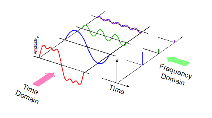
A physical process can be described either in the time domain or frequency domain, which can be represented as a function of time t, i.e., h(t) and a function of frequency, f or angular frequency,ω (ω=2𝜋f), i.e., H(ω), respectively. The two representations of the the functions can transfer back and forth by means of the Fourier transform equations,

In computational work, a continuous function h(t) cannot be given to work with, but the Fourier transform of a function can studied by a finite number of consecutive sampled points.

where Δ is sampling interval, then the integral can be approximate by a discrete sum,

Therefore, the discrete Fourier transform (DFT) of the N points is denoted as

The formula for the discrete inverse Fourier transform is

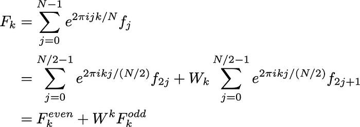
The DFT is n×k elements matrix multiplication process, which appears to be an O(N²) complexity. However, It can be simplified to O(NlogN) complexity operations with an algorithm called the fast Fourier transform (FFT). Danielson-Lanczos Lemma states that a DFT of length N can be rewritten as the sum of an even-numbered and an odd-numbered points DFT of length N/2,

With the restriction on N a power of 2, the data can be transformed recursively all the way down to length 1, which is nothing but one-point transform of the input frequency f. The value of n corresponds to a specific pattern of even and odd in the equation. Thereafter, the structure of an FFT algorithm can be built. First, reordering the data by bit reversal, where butterfly diagram represents. Then an outer loop is executed logN times and calculates transforms of length 2, 4, 8, …, N. For each stage of this process, two nested inner loops are used to implement the Danielson-Lanczos formula. The input array contains N complex time samples in a real array of length 2N, with real and imaginary parts alternating. The output array contains the complex Fourier spectrum at N values of frequency. Real and imaginary parts again alternate.
Denoising Data
The FFT is one of the most important algorithms that have changed the world fundamentally. It offers a computationally fast and efficient way for DFT calculation. It’s a notably piece of technology in digital communication, satellite communication, TV technology, data analysis, audio compression and image compression. It’s also a numerical technique to solve PDEs (partial differential equation) in scientific computing. In data science, the FFT can be used to denoise data. The algorithm is nontrivial but well-known and it’s also well packed in many programming languages, therefore you even don’t bother to know the details under the hood, but you’re still able to implement this tool. In this blog, I will use Python to built a toy model and give a flavor for how the FFT works.
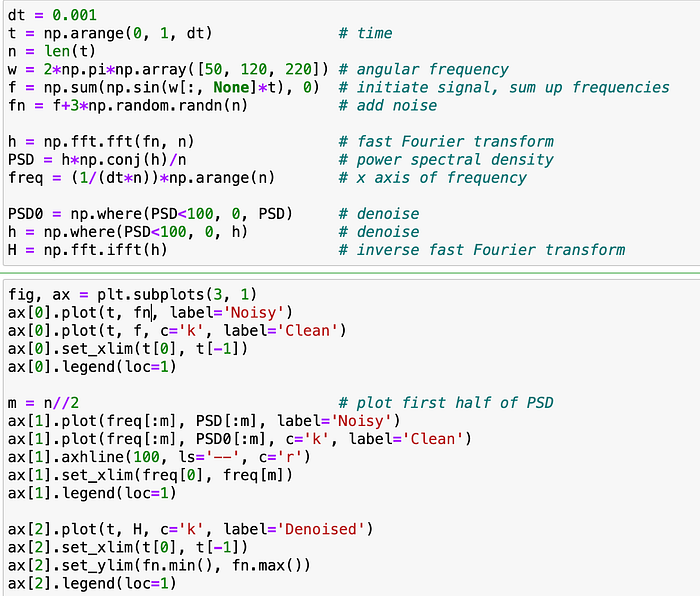
First, I created a simple signal of 3 frequencies with noise, and then I computed the FFT. By observing the power spectral density, I chose my denoising condition. I computed inverse FFT and changed back to time domain.

The first figure shows the original signal and the noisy one in frequency domain. The second figure represents the power spectral density in frequency domain. By cutting off the noise, the denoised frequency is shown in the third figure.

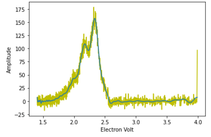
The programming and figures above give basic ideas of the FFT. Be more realistic, another example is shown belown in real world. If the spectrum with heavy noise, the FFT can efficiently clean the data and retrieve a smoothy results we expect.

